User asked to surface system-wide congestion (more accurate than
single-cube), bring back the latency-breakdown plot under a separate
filename, and rename the obscure ``streaming`` category.
Scenarios:
Renamed all_pe_to_pe0 → all_pe_cube0_to_pe0 (clarify cube scope).
Added two SIP-wide scenarios:
sip_local_all — every PE in sip0 (128 total) accesses its own
local slice. All paths disjoint (each PE owns
its own hbm_ctrl.peX), so the model should
scale linearly with cube count.
sip_hotspot_pe0 — every PE in sip0 (128 total) targets
sip0.cube0.pe0_slice. Worst-case hotspot:
UCIe inbound + r0c0→hbm_ctrl.pe0 saturated.
Each bar now carries an ``N=...`` annotation showing the issuer
count, and the chart titles say the scope explicitly.
Effective BW + util at 16 KB:
sip_local_all N=128 eff= 27.2 TB/s util_a= 83 %
sip_hotspot_pe0 N=128 eff= 134 GB/s util_a= 93 %
(UCIe-into-cube0 saturated)
Plots:
no_congestion.png + congestion.png — Effective BW utilization
(two bars: single vs aggregate peak)
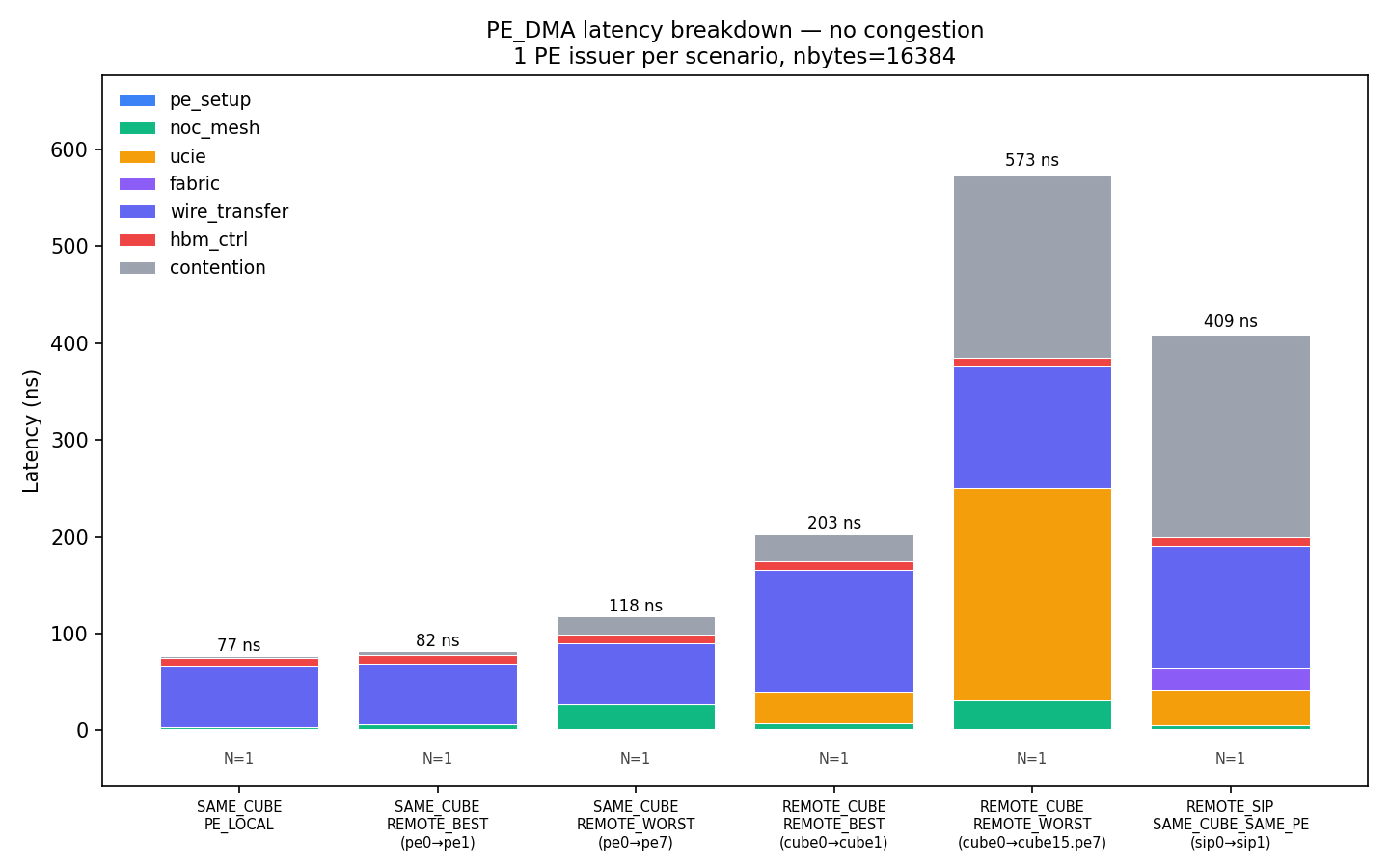
breakdown_no_congestion.png +
breakdown_congestion.png — stacked latency breakdown
(renamed from previous)
summary.csv with columns for both views.
The visual y-cap on BW utilization is 150 %. Bars exceeding it (e.g.
sip_local_all's util_single = 10,639 %) are drawn at the cap with an
upward arrow and the real value annotated. The verification rule for
``util_single`` is loosened to ``≤ n_issuers × 100 % + 5 %`` so
massively-parallel disjoint scenarios pass.
Category renamed: ``streaming`` → ``wire_transfer``. It is the
bulk-transfer time = (n_flits − 1) × flit_bytes / bottleneck_bw — the
cost of streaming the rest of the payload through the slowest wire
after the first flit has arrived.
All checks PASS.
Co-Authored-By: Claude Opus 4.7 (1M context) <noreply@anthropic.com>
64 KiB
1440x900px
64 KiB
1440x900px